Unrolled GANs are a variation of GANs. The problem they try to resolve is -

Problem with GANs that Unrolled GANs try to resolve

They try to stabilize the learning of GANs and thus, leads to convergence. Also, they try to eliminate the problem of mode collapse in vanilla GANs wherein there is little to no variation in the images generated by the generator.

Approach

Consider the loss function $f(\theta_G, \theta_D)$ where $\theta_G$ is the tuple of parameters of the generator and $\theta_D$ is the tuple of parameters of the discriminator.

Let optimal parameters be $\theta_G^* $ and $\theta_D^* $ for generator and discriminator respectively.

Then, using the loss equation of vanilla GANs -

$$\theta_G^* = argmin_{\theta_G} \max_{\theta_D} f(\theta_G, \theta_D) = argmin_{\theta_G} f(\theta_G, \theta_D^* (\theta_G))$$ $$\theta_D^*(\theta_G) = argmax_{\theta_D} f(\theta_G, \theta_D)$$

The main idea presented in this paper is that, the generator just tries to fool the discriminator at this point of time. However, this could lead to oscillation.

An example of such oscillation -

Consider two generator states $\theta_{G_1}$ and $\theta_{G_2}$ and two corresponding discriminator states $\theta_{D_1}$ and $\theta_{D_2}$ respectively. Now, let’s say generator before training, is currently at $\theta_{G_1}$ and the discriminator after training, is at $\theta_{D_1}$. Let the generator after training, go to state $\theta_{G_2}$ which fools the discriminator successfully.

Now, after training the discriminator, let the discriminator go to state $\theta_{D_2}$ and let’s say, due to this, the generator can’t fool it anymore.

Let’s say that generator at state $\theta_{G_1}$ could successfully fool discriminator at state $\theta_{D_2}$. Then, after training the generator again, the generator could go back to state $\theta_{G_1}$ from state $\theta_{G_2}$.

This could lead to an endless oscillation.

So, to avoid such as oscillation, the idea is to train the generator with respect to the approximate discriminator, a few steps into the future.

Consider the following recursive definintion -

$$\theta_D^0 = \theta_D$$ $$\theta_D^{k+1} = \theta_D^k + \eta^k \frac{df(\theta_G, \theta_D^K)}{d \theta_D^k}$$

i.e. the next value of $\theta_D$ is defined by taking a small step of size $\eta^k$ in the direction of increasing $f(\theta_G, \theta_D^k)$. So, $\theta_D^{k+1}$ represents the state of the discriminator if the generator remains constant for k+1 steps and the discriminator is trained for k+1 steps.

So, this is an approximation of the future discriminator.

For training the generator, we use the $f_K(\theta_G, \theta_D)$ defined as follows -

$$f_K(\theta_G, \theta_D) = f(\theta_G, \theta_D^K(\theta_G, \theta_D))$$

where $\theta_D^K$ represents using $\theta_G$ and $\theta_D$ as initial values for the recursive calculation defined above for finding $\theta_D^K$.

This means that the generator is updated using the approximate discriminator function from the future.

However, the discriminator is updated in the same way as vanilla GANs, i.e. using only the current generator. So, the update equations are -

$$\theta_G \leftarrow \theta_G - \eta \frac{df_K(\theta_G, \theta_D)}{d \theta_G}$$ $$\theta_D \leftarrow \theta_D + \eta \frac{df(\theta_G, \theta_D)}{d \theta_D}$$

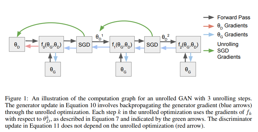
Figure 1 represents the procedure for unrolling in 2 steps. $f_2(\theta_G, \theta_D)$ is computed for training the generator. For finding the gradient, backpropogation through time is required for the discriminator.

However, for updating the discriminator, only gradients from $f_0(\theta_G, \theta_D)$ are considered.

Experiments

A model was trained on a 2D mixture of 8 Gaussians arranged in a circle.

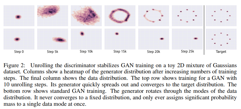
In case of Vanilla GANs, there is a continuous oscillation, which is similar to the example of oscillation given above (only for a larger cycle). Also, there is a mode collapse, since at no time does the generator know about all possibile transformations of latent vector to images. It only knows the transformation corresponding to 1 Gaussian.

However, in case of unrolled GANs, it finally converges and the generator has a complete picture of what the possible transformations are, thus eliminating the problem of mode collapse.

References

• Metz, Poole, et al. “Unrolled Generative Adversarial Networks” CoRR. 2018.