Stacked GANs are top-down stack of GANs, each trained to generate “plausible” lower-level representations conditioned on higher-level representations. Prior to this there was quite success in bottom-up approach of discrimination by CNNs which is learning useful representations from the data, whereas learning top-down generative models will help to explain the data distribution and there was low success for data with large variations with state-of-the-art DNNs was still bad.

Pre-trained encoder

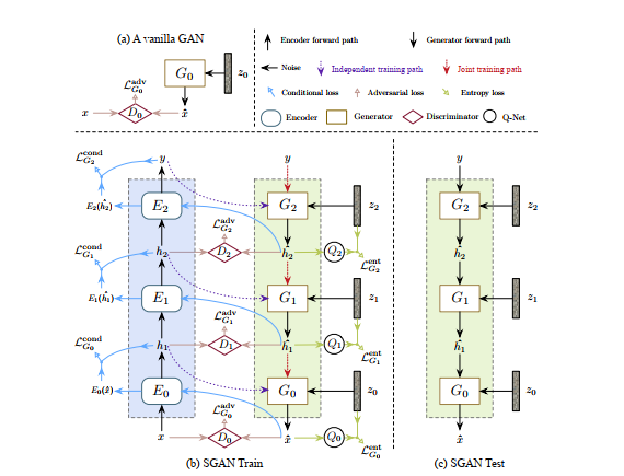
A bottom up DNN pre-trained for classification is referred to as the encoder $E$. Each DNN entails a mapping $h_{i+1}=E_i(h_i)$, where $i\in\{0,1,\ldots, N-1\}$ where $N$ is the number of hierarchies. Each $E_i$ contains a sequence of neural layers. We start with $x=h_0$ and final classification result is $y=h_N$

Stacked Generators

Our goal is to train a top-down generator $G$ that inverts $E$. $G$ consists of a top-down stack of generators $G_i$, each trained to invert $E_i$. $G_i$ takes $\hat h_{i+1}$ and noise vector $z_i$ and gives $\hat h_i=G_i(\hat h_{i+1}, z_i)$.

We first train each GAN independently and then train them jointly in an end-to-end manner.

During training we use $\hat h_i=G(h_{i+1}, z_i)$ and during combined training we use $\hat h_i=G(\hat h_{i+1}, z_i)$. In loss equations we replace $h_{i+1}$ with $\hat h_{i+1}$.

Huang, Xun, et al. describe this as:

Intuitively, the total variations of images could be decomposed into multiple levels, with higher-level semantic variations (e.g., attributes, object categories, rough shapes) and lower-level variations (e.g., detailed contours and textures, background clutters). This allows using different noise variables to represent different levels of variations.

The training procedure is shown in the Figure. Each generator is trained with a linear combination of three loss terms: adversarial loss, conditional loss, and entropy loss with different parametric weights.
${\cal L}_{G_i}=\lambda {\cal L}_{G_i}^{adv}+{\cal L}_{G_i}^{cond}+{\cal L}_{G_i}^{ent}$

For each generator $G_i$ we have a representation discriminator $D_i$ that distinguishes generated representations $\hat h_i$ from real representations $h_i$ . $D_i$ is trained with the loss function:

$$\displaystyle {\cal L}_{D_i}={\mathbb E}_{h_i\sim P_{data, E}}[-\log(D_i(h_i))] + {\mathbb E_{z_i\sim P_{z_i}, h_{i+1}\sim P_{data, E}}}[-\log(1-D_i(G_I(h_{i+1}, z)))]$$

And is trained to fool the representation discriminator with the adversarial loss defined by:

$$\displaystyle {\cal L}_{G_i}^{adv}={\mathbb E}_{h_{i+1}\sim P_{data, E}, z_i\sim P_{z_i}}[-\log(D_i(G_i(h_{i+1}, z)))]​$$

Sampling

To sample images, all $G_i$s are stacked together in a top-down manner, as shown in the Figure. We have the data distribution conditioned on the class label:

$$\displaystyle p_G(\hat x\mid y)=p_G(\hat h_0\mid\hat h_N)\propto p_G(\hat h_0, \hat h_1,\ldots, \hat h_{N-1}\mid \hat h_N)=\prod\limits_{0\le i\le N-1}p_{G_i}(\hat h_i\mid \hat h_{i+1})$$

where each $p_{G_i}(\hat h_i\mid \hat h_{i+1})$ is modeled by a generator $G_i$ . From an information-theoretic perspective, SGAN factorizes the total entropy of the image distribution $H(x)$ into multiple (smaller) conditional entropy terms: $H(x)=H(h_0, h_1, \ldots, h_N)=\sum\limits_{i=0}^{N-1}H(h_i\mid h_{i+1})$, thereby decomposing one difficult task into multiple easier tasks.

Conditional Loss

To prevent $G_i$ from completely ignoring $h_{i+1}$ we use ${\cal L}_{G_i}^{cond}={\mathbb E}_{h_{i+1}\sim p_{\rm data}, z_i\sim p_{z_i}}[f(E_i(G_i(h_{i+1}, z_i)), h_{i+1})]$ where $f$ is an Euclidean distance measure and cross-entropy for labels. This tells us that the generated $\hat h_{i}$ when given to $E_i$ should closely resemble $h_{i+1}$.

Entropy Loss

We would also like to have it not be completely deterministic and sufficiently diverse so we introduce the entropy loss ${\cal L}_{G_i}^{ent}​$. We would want the conditional entropy $H(\hat h_i\mid h_{i+1})​$ to be as high as possible which turns out to be intractable, hence we maximize a variational lower bound on the conditional entropy by using an auxiliary distribution $Q_i(z_i\mid \hat h_i)​$ to approximate the true posterior $p_i(z_i\mid \hat h_i)​$, which gives:

${\cal L}^{ent}_{G_i}={\mathbb E}_{z_i\sim p_{z_i}}[{\mathbb E}_{\hat h_i\sim G_i(\hat h_i\mid z_i)}[-\log Q_i(z_i\mid \hat h_i)]]$ .

It can be proved that minimizing this is equivalent to maximizing a variational lower bound for $H(\hat h_i\mid h_{i+1})$ . In practice we parametrize $Q_i$ with a deep network that predicts the posterior distribution of $z_i$ given $\hat h_i$ . In each iteration we update both $G_i$ and $Q_i$ to minimize ${\cal L}_{G_i}^{ent}$

References

• Huang, Xun, et al. “Stacked Generative Adversarial Networks.” CVPR. Vol. 2. 2017.